Chemprop-RF: A Hybrid Approach to Chemical Property Prediction
Can we combine d-MPNNs and Random Forests to outperform each of them individually?
Whilst neural networks (NNs) have done amazing things with unstructured data such as text and images, they’ve traditionally been outperformed on tabular data by Gradient-Boosted Decision Trees (GBDTs), although recent advances such as TabPFN and TabICL suggest that the performance gap may have closed. I’ve written a bit about TabPFN for chemical datasets here.
One of the most popular deep learning architectures for chemical property prediction is Chemprop, developed by researchers at MIT. A Chemprop model is made up of two NNs. The first is a directed Message Passing Neural Network (d-MPNN), a type of Graph Convolutional Neural Network (GCNN), that takes a graphical representation of a molecule and converts it to a molecular embedding, a vector that describes the original molecule. This molecular embedding is then put through a Feed-Forward Neural Network (FFN), a fully connected NN used to make the final prediction. The model is trained end-to-end, with both NNs being updated at the same time to minimise a loss function.
Once the model is trained, the d-MPNN can be used to calculate a molecular embedding for a collection of molecules. This is a learned representation optimised for the specific chemical prediction problem. This learned representation is a vector with a length equal to the number of input nodes in the FFN. This is very similar to a traditional molecular fingerprint, such as a Morgan fingerprint.
A collection of these learned fingerprints forms a 2-dimensional array, which is tabular data. Since GBDTs regularly outperform NNs on tabular data, can we improve the performance of Chemprop by replacing the FFN with a GBDT after training the d-MPNN?
Whilst writing this post, a paper was published in The Journal of Chemical Information and Modeling by Pat Walters et al., Practically Significant Method Comparison Protocols for Machine Learning in Small Molecule Drug Discovery. This is probably my favourite cheminformatics paper so far this year, with comprehensive guidelines on how to compare machine learning models in a statistically robust way. I’ve tried to follow these recommendations when comparing models here.
Below I compare three models: the first is a Random Forest (this is not gradient-boosted, but provides a good baseline without hyperparameter tuning) trained on Morgan fingerprints; the second is a standard Chemprop model; and the third generates learned fingerprints using the Chemprop d-MPNN and then trains a Random Forest model on these. I used two datasets, one for a classification problem and one for a regression problem. The classification data is the Bile Salt Export Pump dataset and the regression data is the Polaris LogS dataset, both ideas ‘borrowed’ from Practical Cheminformatics posts.
Imports
import subprocess
from collections import defaultdict
from pathlib import Path
from typing import Callable

import matplotlib.pyplot as plt
import numpy as np
import pandas as pd
import seaborn as sns
from numpy.typing import NDArray
from rdkit import Chem
from rdkit.Chem import rdFingerprintGenerator
from scipy.stats import f_oneway
from sklearn.base import BaseEstimator
from sklearn.ensemble import RandomForestClassifier, RandomForestRegressor
from sklearn.metrics import (
    matthews_corrcoef,
    mean_absolute_error,
    r2_score,
    root_mean_squared_error,
)
from sklearn.model_selection import ShuffleSplit
from statsmodels.stats.multicomp import pairwise_tukeyhsd
from tqdm.notebook import tqdm

from visualisation import confusion_matricies, scatter_plots
Useful functions
The first function prepare_data takes the path to a CSV file, creates RDKit molecular objects, removes any that are causing issues, and calculates the Morgan fingerprints for each model.
The second, save_data_for_chemprop, formats the data and saves it for training Chemprop models.
The next three functions: train_chemprop_model, make_chemprop_predictions, and calculate_chemprop_fingerprints, all use subprocess to call the Chemprop CLI. I’ve generally found it easier to use than the Chemprop Python module.
The next two: train_morgan_sklearn_model and train_chemprop_sklearn_model, use Scikit-learn to train Random Forest models, the first using the previously generated Morgan fingerprints, and the second uses the Chemprop learned fingerprints.
Finally, gather_predictions uses all of the trained models to make predictions on a test dataset.
def prepare_data(
    data_path: Path, smiles_col: str, target_col: str
) -> tuple[pd.DataFrame, pd.DataFrame]:
    """Load and clean data, generate Morgan fingerprints.

    Args:
        data_path (Path): Path to CSV file containing data.
        smiles_col (str): Name of the column containing SMILES strings.
        target_col (str): Name of the column containing target variable.

    Returns:
        tuple[pd.DataFrame, pd.DataFrame]: Cleaned dataframe and dataframe of Morgan
                                           fingerprints.
    """
    df = pd.read_csv(data_path)
    df["ROMol"] = df[smiles_col].apply(lambda x: Chem.MolFromSmiles(x))
    df.dropna(subset=["ROMol"], inplace=True)
    mfpgen = rdFingerprintGenerator.GetMorganGenerator(radius=2, fpSize=2048)
    fps = [mfpgen.GetFingerprint(mol) for mol in df["ROMol"]]
    fps_df = pd.DataFrame(np.array(fps))
    df = df[[smiles_col, target_col]]
    return df, fps_df


def save_data_for_chemprop(
    data: pd.DataFrame,
    project_name: str,
    train_idx: NDArray[np.int64],
    test_idx: NDArray[np.int64],
    seed: int,
    fold_number: int,
) -> None:
    """Save training and test data for Chemprop CLI.

    Args:
        data (pd.DataFrame): Dataframe containing data.
        project_name (str): Name of the project.
        train_idx (NDArray[np.int64]): List of indices for training data.
        test_idx (NDArray[np.int64]): List of indices for test data.
        seed (int): Random seed used for splitting data.
        fold_number (int): Fold number for cross-validation.
    """
    Path(f"data/{project_name}/seed_{seed}/fold_{fold_number}/").mkdir(
        parents=True, exist_ok=True
    )
    data.iloc[train_idx].to_csv(
        f"data/{project_name}/seed_{seed}/fold_{fold_number}/train.csv", index=False
    )
    data.iloc[test_idx].to_csv(
        f"data/{project_name}/seed_{seed}/fold_{fold_number}/test.csv", index=False
    )


def train_chemprop_model(
    project_name: str, seed: int, fold_number: int, task_type: str
) -> None:
    """Train Chemprop model using CLI.

    Args:
        project_name (str): Name of the project.
        seed (int): Random seed used for splitting data.
        fold_number (int): Fold number for cross-validation.
        task_type (str): Type of task ('classification' or 'regression').
    """
    subprocess.run(
        [
            "chemprop",
            "train",
            "--data-path",
            f"data/{project_name}/seed_{seed}/fold_{fold_number}/train.csv",
            "--task-type",
            task_type,
            "--output-dir",
            f"models/{project_name}/seed_{seed}/fold_{fold_number}",
        ],
        check=True,
        stdout=subprocess.DEVNULL,
        stderr=subprocess.DEVNULL,
    )


def make_chemprop_predictions(project_name: str, seed: int, fold_number: int) -> None:
    """Make predictions using trained Chemprop model.

    Args:
        project_name (str): Name of the project.
        seed (int): Random seed used for splitting data.
        fold_number (int): Fold number for cross-validation.
    """
    subprocess.run(
        [
            "chemprop",
            "predict",
            "--test-path",
            f"data/{project_name}/seed_{seed}/fold_{fold_number}/test.csv",
            "--model-paths",
            f"models/{project_name}/seed_{seed}/fold_{fold_number}/",
            "--preds-path",
            f"data/{project_name}/seed_{seed}/fold_{fold_number}/preds.csv",
        ],
        check=True,
        stdout=subprocess.DEVNULL,
        stderr=subprocess.DEVNULL,
    )


def calculate_chemprop_fingerprints(
    project_name: str, seed: int, fold_number: int, dataset_type: str
) -> None:
    """Calculate Chemprop fingerprints using trained Chemprop model.

    Args:
        project_name (str): Name of the project.
        seed (int): Random seed used for splitting data.
        fold_number (int): Fold number for cross-validation.
        dataset_type (str): Type of dataset ('train' or 'test').
    """
    subprocess.run(
        [
            "chemprop",
            "fingerprint",
            "--test-path",
            f"data/{project_name}/seed_{seed}/fold_{fold_number}/{dataset_type}.csv",
            "--output",
            f"data/{project_name}/seed_{seed}/fold_{fold_number}/{dataset_type}_fps.csv",
            "--model-path",
            f"models/{project_name}/seed_{seed}/fold_{fold_number}/",
            "--ffn-block-index",
            "0",
        ],
        check=True,
        stdout=subprocess.DEVNULL,
        stderr=subprocess.DEVNULL,
    )


def train_morgan_sklearn_model(
    fps_df: pd.DataFrame, y: pd.Series, train_idx: NDArray[np.int64], task_type: str
) -> BaseEstimator:
    """Train Scikit-learn model using Morgan fingerprints.

    Args:
        fps_df (pd.DataFrame): Dataframe of Morgan fingerprints.
        y (pd.Series): Series of target variable.
        train_idx (NDArray[np.int64]): List of indices for training data.
        task_type (str): Type of task ('classification' or 'regression').

    Returns:
        BaseEstimator: Trained Scikit-learn model.
    """
    if task_type == "regression":
        rf = RandomForestRegressor(n_estimators=100, random_state=0)
    else:
        rf = RandomForestClassifier(n_estimators=100, random_state=0)
    X_train = fps_df.iloc[train_idx]
    y_train = y.iloc[train_idx]
    return rf.fit(X_train, y_train)


def train_chemprop_sklearn_model(
    project_name: str,
    seed: int,
    fold_number: int,
    y: pd.Series,
    train_idx: NDArray[np.int64],
    task_type: str,
) -> BaseEstimator:
    """Train Scikit-learn model using Chemprop fingerprints.

    Args:
        project_name (str): Name of the project.
        seed (int): Random seed used for splitting data.
        fold_number (int): Fold number for cross-validation.
        y (pd.Series): Series of target variable.
        train_idx (NDArray[np.int64]): List of indices for training data.
        task_type (str): Type of task ('classification' or 'regression').

    Returns:
        BaseEstimator: Trained Scikit-learn model.
    """
    X_train = pd.read_csv(
        Path(f"data/{project_name}/seed_{seed}/fold_{fold_number}/train_fps_0.csv")
    )
    if task_type == "regression":
        rf = RandomForestRegressor(n_estimators=100, random_state=0)
    else:
        rf = RandomForestClassifier(n_estimators=100, random_state=0)
    y_train = y.iloc[train_idx]
    return rf.fit(X_train, y_train)


def gather_predictions(
    morgan_rf: BaseEstimator,
    chemprop_rf: BaseEstimator,
    project_name: str,
    seed: int,
    fold_number: int,
    df: pd.DataFrame,
    fps_df: pd.DataFrame,
    test_idx: NDArray[np.int64],
    target_col: str,
    task_type: str,
) -> dict:
    """Gather predictions from all models.

    Args:
        morgan_rf (BaseEstimator): Trained Scikit-learn model on Morgan fingerprints.
        chemprop_rf (BaseEstimator): Trained Scikit-learn model on Chemprop fingerprints.
        project_name (str): Name of the project.
        seed (int): Random seed used for splitting data.
        fold_number (int): Fold number for cross-validation.
        df (pd.DataFrame): Dataframe containing data.
        fps_df (pd.DataFrame): Dataframe of Morgan fingerprints.
        test_idx (NDArray[np.int64]): List of indices for test data.
        target_col (str): Name of the column containing target variable.
        task_type (str): Type of task ('classification' or 'regression').

    Returns:
        dict: Updated dictionary with predictions.
    """
    predictions = {}
    rf_preds = morgan_rf.predict(fps_df.iloc[test_idx])
    chemprop_rf_preds = chemprop_rf.predict(
        pd.read_csv(
            f"data/{project_name}/seed_{seed}/fold_{fold_number}/test_fps_0.csv"
        )
    )
    chemprop_probas = pd.read_csv(
        f"data/{project_name}/seed_{seed}/fold_{fold_number}/preds.csv"
    )[target_col]
    if task_type == "regression":
        chemprop_preds = chemprop_probas
    else:
        chemprop_preds = (chemprop_probas >= 0.5).astype(int)
    y_true = df.iloc[test_idx][target_col]
    predictions[f"seed_{seed}_fold_{fold_number}"] = {
        "rf": rf_preds,
        "chemprop_rf": chemprop_rf_preds,
        "chemprop": chemprop_preds,
        "true": y_true,
    }
    return predictions
To compare the models, I used 5x5 cross-validation. This approach involves using five different random seeds to generate data splits for 5-fold cross-validation, resulting in 25 unique train-test splits. For each split, the models are trained on the training data and then used to make predictions on the test data.
def run_model_comparison(
    data_path: Path,
    project_name: str,
    smiles_col: str,
    target_col: str,
    task_type: str,
    n_seeds: int = 5,
    n_folds: int = 5,
    test_frac: float = 0.2,
) -> dict:
    """Run model comparison pipeline.

    Args:
        data_path (Path): Path to CSV file containing data.
        project_name (str): Name of the project.
        smiles_col (str): Name of the column containing SMILES strings.
        target_col (str): Name of the column containing target variable.
        task_type (str): Type of task ('classification' or 'regression').
        n_seeds (int, optional): Number of random seeds for cross-validation. Defaults to 5.
        n_folds (int, optional): Number of folds for cross-validation. Defaults to 5.
        test_frac (float, optional): Fraction of data to use as test set. Defaults to 0.2.

    Returns:
        dict: Dictionary containing predictions from all models.
    """
    df, fps_df = prepare_data(data_path, smiles_col, target_col)

    all_predictions = {}
    for seed in tqdm(range(n_seeds), total=n_seeds, desc="Seeds", unit="seed"):
        cv = ShuffleSplit(n_splits=n_folds, test_size=test_frac, random_state=seed)
        for fold_number, (train_idx, test_idx) in tqdm(
            enumerate(cv.split(df)),
            total=n_folds,
            desc=f"Seed {seed}: Folds",
            unit="fold",
        ):
            # Save data for training models using Chemprop CLI
            save_data_for_chemprop(
                df, project_name, train_idx, test_idx, seed, fold_number
            )

            # Train Chemprop model using CLI
            train_chemprop_model(project_name, seed, fold_number, task_type)

            # Make predictions on test set using trained Chemprop model
            make_chemprop_predictions(project_name, seed, fold_number)

            # Use trained model to create fingerprints
            calculate_chemprop_fingerprints(project_name, seed, fold_number, "train")
            calculate_chemprop_fingerprints(project_name, seed, fold_number, "test")

            # Train Scikit-learn models on Morgan fingerprints
            morgan_rf = train_morgan_sklearn_model(
                fps_df, df[target_col], train_idx, task_type
            )

            # Train Scikit-learn model on Chemprop fingerprints
            chemprop_rf = train_chemprop_sklearn_model(
                project_name,
                seed,
                fold_number,
                df[target_col],
                train_idx,
                task_type,
            )

            # Gather predictions
            predictions = gather_predictions(
                morgan_rf,
                chemprop_rf,
                project_name,
                seed,
                fold_number,
                df,
                fps_df,
                test_idx,
                target_col,
                task_type,
            )
            all_predictions.update(predictions)
    return all_predictions
The next two cells run the training and prediction process for the classification and regression datasets.
# Set up workspace
Path("data").mkdir(exist_ok=True)
Path("models").mkdir(exist_ok=True)
np.random.seed(42)

n_seeds = 5
n_folds = 5
test_frac = 0.2
data_path = Path("data/raw/bsep.csv")
project_name = "bsep"
smiles_col = "smiles"
target_col = "bsep"
task_type = "classification"

classification_predictions = run_model_comparison(
    data_path,
    project_name,
    smiles_col,
    target_col,
    task_type,
    n_seeds=n_seeds,
    n_folds=n_folds,
    test_frac=test_frac,
)
Seeds:   0%|          | 0/5 [00:00<?, ?seed/s]
Seed 0: Folds:   0%|          | 0/5 [00:00<?, ?fold/s]
Seed 1: Folds:   0%|          | 0/5 [00:00<?, ?fold/s]
Seed 2: Folds:   0%|          | 0/5 [00:00<?, ?fold/s]
Seed 3: Folds:   0%|          | 0/5 [00:00<?, ?fold/s]
Seed 4: Folds:   0%|          | 0/5 [00:00<?, ?fold/s]
n_seeds = 5
n_folds = 5
test_frac = 0.2
data_path = Path("data/raw/biogen_logS.csv")
project_name = "logS"
smiles_col = "SMILES"
target_col = "logS"
task_type = "regression"

regression_predictions = run_model_comparison(
    data_path,
    project_name,
    smiles_col,
    target_col,
    task_type,
    n_seeds=n_seeds,
    n_folds=n_folds,
    test_frac=test_frac,
)
Seeds:   0%|          | 0/5 [00:00<?, ?seed/s]
Seed 0: Folds:   0%|          | 0/5 [00:00<?, ?fold/s]
Seed 1: Folds:   0%|          | 0/5 [00:00<?, ?fold/s]
Seed 2: Folds:   0%|          | 0/5 [00:00<?, ?fold/s]
Seed 3: Folds:   0%|          | 0/5 [00:00<?, ?fold/s]
Seed 4: Folds:   0%|          | 0/5 [00:00<?, ?fold/s]
The next function takes the predicted values and true values from the test set and calculates a relevant performance metric.
For the moderately imbalanced BSEP classification data (17% positive class), I used the Matthews Correlation Coefficient (MCC). MCC is a value between -1 and 1 and is a robust metric for imbalanced datasets. For the LogS regression data, I used the coefficient of determination (R2). An R2 value of 1 indicates perfect agreement between predicted and true values, with no lower limit for poor predictions.
def calculate_performance(preds_dict: dict, metric: Callable) -> dict:
    """Analyse performance of models.

    Args:
        preds_dict (dict): Dictionary containing predictions from all models.
        metric (Callable): Metric function to evaluate performance.

    Returns:
        dict: Dictionary containing performance metrics for each model.
    """
    metrics = defaultdict(list)
    for predictions in preds_dict.values():
        metrics[f"rf_{metric.__name__}"].append(
            metric(predictions["true"], predictions["rf"])
        )
        metrics[f"chemprop_rf_{metric.__name__}"].append(
            metric(predictions["true"], predictions["chemprop_rf"])
        )
        metrics[f"chemprop_{metric.__name__}"].append(
            metric(predictions["true"], predictions["chemprop"])
        )
    return metrics


classification_metrics = calculate_performance(
    classification_predictions, matthews_corrcoef
)

regression_metrics = calculate_performance(regression_predictions, r2_score)
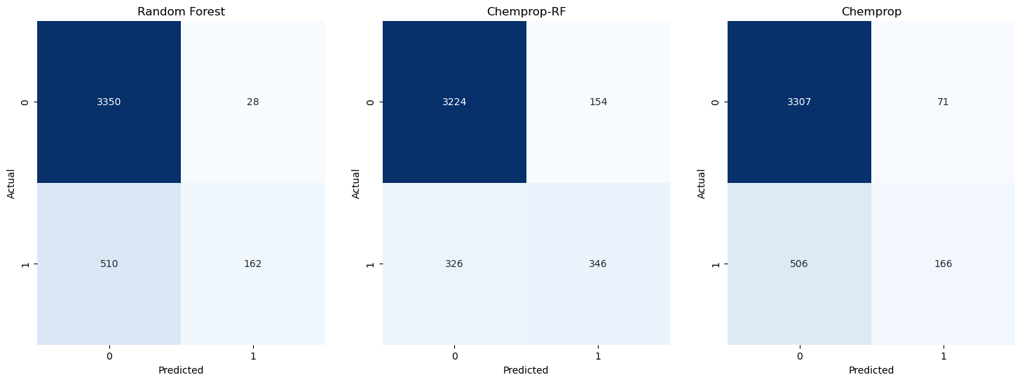
To visualise and inspect the classification results, I’ve used confusion matricies. All three models have a significant number of True Negatives (TN) in the top left square. The Random Forest model and the Chemprop model have a significant number of False Negatives (FN), whereas the Chemprop-RF model has more True Positives (TP) and more False Positives (FP).
confusion_matricies(classification_predictions)
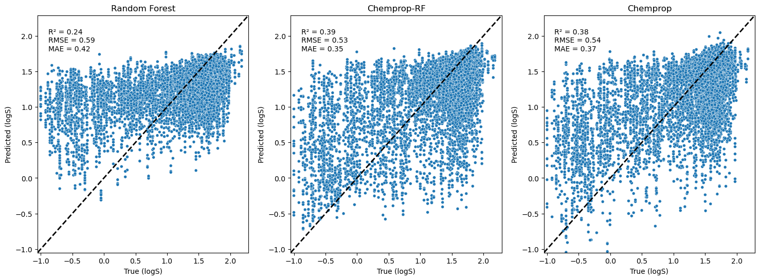
To visualise and inspect the regression results, I’ve used x-y scatter plots of the predicted values against the true values. The Random Forest regressor has poor predictions, with more values being overestimated. The Chemprop model and the Chemprop-RF models perform better, especially on these lower LogS values. Some performance metrics are annotated on the plots in the top left: R2, RMSE (root mean squared error), and MAE (mean absolute error).
scatter_plots(regression_predictions)
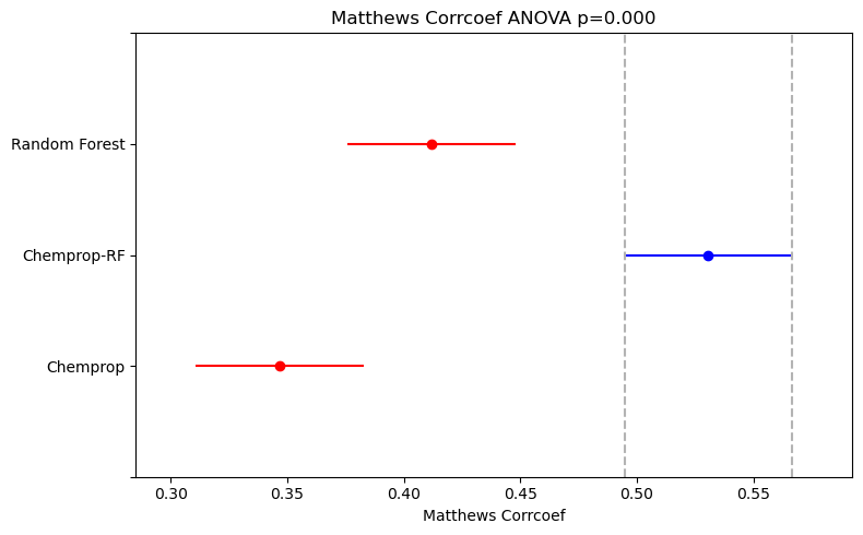
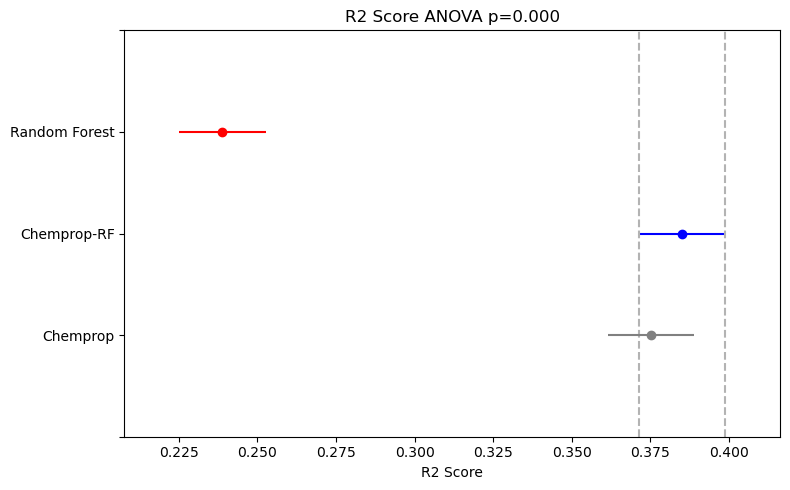
As recommended in the paper I’ve linked, I used one-way ANOVA to compare the performance distributions from the 5x5 cross-validation and determine if there was a statistically significant difference between the means. This was followed by Tukey’s Honest Significant Differences as a post-hoc pairwise test. The results are plotted using the Simultaneous Confidence Interval plot from the statsmodels Python library.
For both the classification and regression datasets, the ANOVA results showed a statistically significant difference in model performance (p<0.05).
For the classification dataset, post-hoc tests revealed a statistically significant difference in performance between all pairs of models, with the Chemprop-RF model performing the best.
For the regression dataset, the Random Forest model performed statistically significantly worse than the other two. However, there was no statistically significant difference between the performance of the Chemprop and Chemprop-RF models.
The classification dataset (BSEP, 807 entries) is much smaller than the regression dataset (LogS, 2,173 entries). This might suggest that Chemprop-RF models are particularly effective for low-data problems, where there isn’t enough data to train a high-performing Feed-Forward Neural Network (FFN) alone.
# Adapted from https://github.com/PatWalters/practical_cheminformatics_posts/blob/main/adme_comparison/
def run_anova(df_in: pd.DataFrame, col: str) -> float:
    """Run one-way ANOVA on model performance."""
    res_list = []
    for _, v in df_in.groupby("method"):
        res_list.append(v[col].values)
    return f_oneway(*res_list)[1]


def plot_metric_comparison(metric_dict: dict, metric: Callable) -> None:
    """Plot comparison of model performance using a specified metric.

    Args:
        metric_dict (dict): Dictionary containing performance metrics for each model.
        metric (Callable): Metric function used to evaluate performance.
    """
    _, ax = plt.subplots()
    melt_df = pd.DataFrame(metric_dict).melt()
    melt_df["method"] = melt_df.variable.map(
        {
            f"rf_{metric.__name__}": "Random Forest",
            f"chemprop_rf_{metric.__name__}": "Chemprop-RF",
            f"chemprop_{metric.__name__}": "Chemprop",
        }
    )
    best_model = (
        melt_df.groupby("method")["value"]
        .mean()
        .reset_index()
        .sort_values("value", ascending=False)
        .method.values[0]
    )
    tukey = pairwise_tukeyhsd(
        endog=melt_df["value"], groups=melt_df["method"], alpha=0.05
    )
    tukey.plot_simultaneous(comparison_name=best_model, ax=ax, figsize=(8, 5))
    anova_p_value = run_anova(melt_df, "value")
    ax.set_title(
        f"{metric.__name__.replace('_', ' ').title()} " + f"ANOVA p={anova_p_value:.3f}"
    )
    ax.set_xlabel(f"{metric.__name__.replace('_', ' ').title()}")

    plt.tight_layout()
    plt.show()


plot_metric_comparison(classification_metrics, matthews_corrcoef)
plot_metric_comparison(regression_metrics, r2_score)